Physics

Physical components of Longterm

1: Vegetation
2: Weathering
3: Sea Level

This section and its subsections are incomplete. For a complete description of the physics, see the paper.

The Longterm Climate Model is a box model with three types of prognostic boxes: ocean, soil, and vegetation. The Longterm logo depicts these boxes in its default configuration. In every configuration, there are two ocean boxes, colored blue in the logo. In the default configuration, there are three vegetation boxes, shown in green, and two soil boxes, shown in brown.

Longterm integrates $6 + n_\mathrm{veg} + n_\mathrm{soil}$ prognostic variables, where $n_\mathrm{veg}$ and $n_\mathrm{soil}$ are the numbers of vegetation and soil boxes, respectively. Therefore, in the default configuration of $n_\mathrm{veg} = 3$ and $n_\mathrm{soil} = 2$, there are 11 prognostic variables: two for temperature, two for alkalinity, and seven for carbon. These variables are distributed among boxes as follows:

Box	Carbon	Temperature	Alkalinity
Surface ocean	x	x	x
Deep ocean	x
Vegetation	x
Soil	x

The surface-ocean box is slightly special with regards to carbon. Its carbon variable represents not just the mass of carbon in the surface ocean, but the total mass of carbon in the surface ocean and the atmosphere. The carbon is partitioned between them diagnostically and the temperature of the atmosphere is set to 10 K above the temperature of the surface ocean.

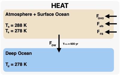
The model physics determines the flows of heat, carbon, and alkalinity through these boxes. The sources and sinks of heat for the surface ocean are: radiative forcing from greenhouse gases (CO$_2$ only), radiative forcing from planetary albedo (sensitive to vegetation only), radiative forcing from intrinsic feedbacks (e.g., Planck, water vapor, and lapse rate all rolled up into one number), and downwelling (and associated upwelling) of water to (from) the deep ocean.

The flows of heat and preindustrial temperatures of the two ocean boxes.

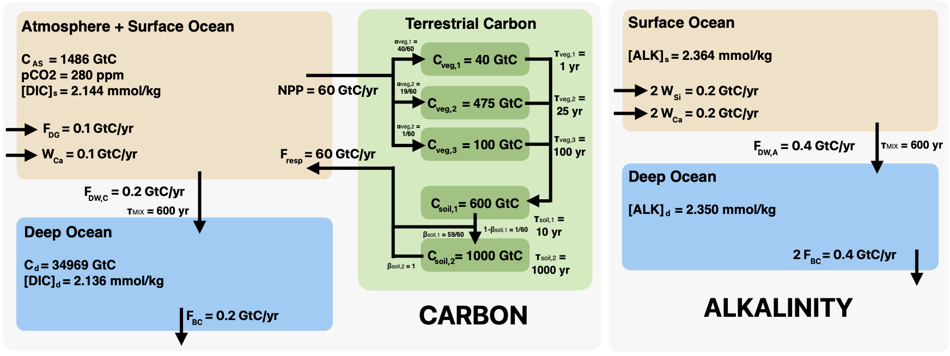
The flows of alkalinity, expressed below in terms of equivalent mass of carbon, are from weathering of terrestrial silicates and carbonates to the surface ocean, downwelling from the surface ocean to the deep ocean, and burial of carbonates on the ocean floor. The flows of carbon are the most complicated. The surface ocean and atmosphere gain carbon from degassing (e.g., volcanoes) and from the weathering of terrestrial carbonates, and they lose carbon via downwelling to the deep ocean. The surface oceana and atmosphere also lose carbon through the net primary productivity of terrestrial vegetation and gain carbon from respiration in soils. The movement of carbon between vegetation and soil pools is governed by decay timescales and preindustrial stocks that can be set by the user. Finally, the deep ocean loses carbon via burial of carbonates on the ocean floor.

The physics governing the flows of heat, carbon, and alkalinity are described in the pages below.

1 - Vegetation

Vegetation and soil physics

By default, the terrestrial carbon scheme contains three pools of live vegetation and two soil pools. The number of vegetation and soil pools can be modified at runtime, but the default settings are designed to approximate the flows, stocks, and turnover times of carbon in Earth’s vegetation and soils.

Conceptually, the movement of carbon through these pools is handled by Longterm as follows. The global net primary productivity (NPP) is a function of the atmospheric CO₂ concentration, and fixed fractions of that NPP flow into each of the respective pools of vegetative carbon. Each of those pools has a residence time for its carbon, with the rate of outflow (representing shedding and mortality) governed by first-order kinetics. The vegetative carbon pools operate in parallel, each receiving its designated fraction of NPP and each losing carbon at a rate proportional to its stock.

Although global NPP is specified as a function of atmospheric concentration of CO₂, the fraction of NPP that goes to each vegetation carbon pool is fixed. For example, in the default preindustrial steady state, 1 PgC/yr out of 60 PgC/yr total NPP goes to the 100-year carbon pool; therefore, whatever the value of the global NPP evolves to be in the climate simulation, 1/60 of the NPP will flow to that 100-year pool. The governing equation for the mass of carbon in vegetation pool $i$ is

$$ dC_{\mathrm{veg},i}/dt = \alpha_{\mathrm{veg},i} \mathrm{NPP} - C_{\mathrm{veg},i}/\tau_{\mathrm{veg},i} \, . $$

The first term on the right-hand side represents the net fixing of carbon by the vegetation through photosynthesis, with $\alpha_{\mathrm{veg},i}$ being the fraction of NPP destined for carbon pool $i$ (e.g., 1/60 for the 100-yr pool in the default configuration). The second term on the right-hand side represents the movement of carbon from live biomass to dead biomass via plant mortality and shedding of leaves, branches, and similar material.

Default Timescale (yr)	Default PI Carbon (GtC)	Default PI NPP (GtC/yr)	Represents
100	100	1	Boreal forest’s slow pool
25	475	19	Tropical and temperate forests’ slow pools
1	40	40	All forests’ fast pools

The net primary productivity (NPP) is a function of the atmospheric CO$_2$ concentration,

$$ \mathrm{NPP} = \mathrm{NPP}_\mathrm{max} \frac{\left(\frac{[\mathrm{CO}_2]}{[\mathrm{CO}_2]_0}\right)^2} {\frac{\mathrm{NPP}_\mathrm{max}}{\mathrm{NPP}_0} - 1 + \left(\frac{[\mathrm{CO}_2]}{[\mathrm{CO}_2]_0}\right)^2} \, , $$

where [CO₂] is the atmospheric concentration of CO₂, [CO₂]₀ is the corresponding preindustrial value, and NPP₀ is the preindustrial net primary productivity. The maximum NPP achieved when the CO₂ concentration is high enough to not be a limiting factor. The preindustrial value of net primary productivity, NPP₀, is determined by summing the preindustrial vegetation carbon masses divided by their decay timescales. As NPP deviates from NPP₀, it is apportioned among the vegetation carbon pools in the same proportions.

Although the vegetative pools operate in parallel, the soil pools operate in serial. All vegetative pools decay to the first soil pool, which represents a combination of woody debris, litter, and near-surface soil. The loss of carbon from that soil pool is governed by first-order kinetics with a residence time that is sensitive to the global mean temperature T_s. The outflows from the soil pool are partitioned into two destinations: a constant fraction of the outflow is oxidized and sent directly to the atmosphere, with the remaining outflow sent to the next soil pool. This cascade continues to the last soil pool, which sends all of its outflow of carbon to the atmosphere.

The rate at which soil carbon decays, moving to the next soil pool and/or to the atmosphere as CO₂, is set by a timescale $\tau$_soil that depends on global-mean temperature according to a Q₁₀ value,

$$ \tau_\mathrm{soil} = \tau_{\mathrm{soil},0}\, Q_{10}^{-(T_{\mathrm{atmo}}-T_{\mathrm{atmo},0})/(10\,\mathrm{K})}\, , $$

with a default value of Q₁₀ = 1.5 and with default values of $\tau$_soil,0 for each soil pool as given in the table below.

Default Timescale (yr)	Default PI Carbon (GtC)	Default Fraction that Decays to Atmosphere
1000	1000	1
10	600	59/60

2 - Weathering

Weathering and burial of carbonates and silicates

Terrestrial weathering of carbonate and silicate rock is represented by F_wc and F_ws, which are the rates of carbon consumed from the atmosphere by the weathering of carbonate and silicate rock, respectively. These rates are dependent on temperature as

$$ \begin{align*} F_{wc} &= F_{wc,0}\, e^{a_c (T_{\mathrm{surf}}-T_{\mathrm{surf},0})} \\ F_{ws} &= F_{ws,0}\, e^{a_s (T_{\mathrm{surf}}-T_{\mathrm{surf},0})} \, , \end{align*} $$

where F_wc,0 and F_ws,0 are the preindustrial weathering rates, T_surf,0 is the preindustrial surface-ocean temperature, and a_c and a_s are the rates of relative change in the weathering rates per degree of warming (set by constants$dFwcdlogT and constants$dFwsdlogT with default values of 0.10/K and 0.02/K, respectively). Since the global mean surface-air temperature is set diagnostically as the surface-ocean temperature plus a fixed increment, these equations are identical to

$$ \begin{align*} F_{wc} &= F_{wc,0}\, e^{a_c (T_{\mathrm{atmo}}-T_{\mathrm{atmo},0})} \\ F_{ws} &= F_{ws,0}\, e^{a_s (T_{\mathrm{atmo}}-T_{\mathrm{atmo},0})} \, . \end{align*} $$

The rate of carbon burial on the ocean floor in the form of calcium carbonate, \eqn{F_{bc}}{F_bc}, is linear in the concentration of deep-ocean carbonate ion,

$$ F_{bc} = F_{bc,0} + a \left([\mathrm{CO}_3^{2-}] - [\mathrm{CO}_3^{2-}]_0\right) \, , $$

where [CO₃^2-] is the concentration (with dimensions of mol/kg) of carbonate ion in the deep ocean, [CO₃^2-]₀ is its preindustrial value, and a is a constant set to 2.5 x 10¹⁷ kg/yr.

3 - Sea Level

Governing equation for sea level

The committed sea-level rise (CSL; dimensions of m) is the sea-level anomaly relative to preindustrial to which the ocean would equilibrate if the global-mean temperature anomaly were held constant. The CSL is approximated as linear in global-mean temperature with a default slope of 6 m/K. The sea level anomaly (SL; dimensions of m) is the sea-level relative to preindustrial. The evolution of SL is approximated as a relaxation towards CSL with a timescale $\tau$_SL,

$$ \frac{d\mathrm{SL}}{dt} = \min\Big[ \mathrm{SL}_{\mathrm{max}}, (\mathrm{CSL} - \mathrm{SL})/\tau_{\mathrm{SL}} \Big] \, , $$

where SL_max is the maximum sea-level anomaly. The default values of $\tau$_SL and SL_max are 2000 yr and 60 m, respectively.