Get Longterm up and running in under 5 minutes!
New users should read the Overview, Installation, and Examples for a quick start.
This is the multi-page printable view of this section. Click here to print.
Get Longterm up and running in under 5 minutes!
New users should read the Overview, Installation, and Examples for a quick start.
The Longterm Climate Model is a box model with three types of prognostic boxes: ocean, soil, and vegetation. The Longterm logo depicts these boxes in its default configuration. In every configuration, there are two ocean boxes, colored blue in the logo. In the default configuration, there are three vegetation boxes, shown in green, and two soil boxes, shown in brown.
The Longterm logo depicts two ocean boxes (blue), three vegetation boxes (green), and two soil boxes (brown).
Installing and using Longterm in R or Python is easy. Get started in less than 5 minutes:
Installation the longterm package in R or Python is simple.
# From inside R, run:
install.packages("longterm")
# At the terminal, run:
pip install longtermSo is loading longterm and running a simulation.
library(longterm)
output <- longterm()
import longterm
output = longterm.run()Running this command will cause the following plots to display.

The simulation above is boring because we have not specified any perturbations to the climate system. For more interesting simulations, see Examples.
Running longterm with no arguments is boring because it will generate a time series representing a continuation of the preindustrial steady state. Below are some examples of more interesting simulations.
This simulation turns on a 1 W/m2 top-of-atmosphere radiative forcing at t=0 and holds it on for all time thereafter.
output <- longterm(sources=list(rad=1))output = longterm.run(sources={"rad":1})
This simulation turns on a -500 W/m2 top-of-atmosphere radiative forcing at t=0 that then decays with an e-folding timescale of 5 years, representing the effects of a severe nuclear winter.
output <- longterm(sources=list(rad=function(t){ -500*(1-exp(-t/5)) }))import math
output = longterm.run(sources={"rad": lambda t: -500*(1-math.exp(-t/5))})
This simulation releases 5000 GtC of fossil carbon into the atmosphere as CO2 at t=0.
output <- longterm(sources=list(Cas=function(t){ if (t>0) { 5000 } else { 0 } }))output = longterm.run(sources={"Cas": lambda t: 5000 if t > 0 else 0})
longterm functionThe Longterm Climate Model can be run with no arguments as follows.
output <- longterm()output = longterm.run();This, however, is a boring use of longterm, as it will simply return the steady-state preindustrial climate. More interesting simulations are generated by setting some of the optional arguments, especially sources. For example, you could run a simulation in which a 1 W/m2 top-of-atmosphere radiative forcing is turned on and kept on.
output <- longterm(sources(rad=1))output = longterm.run(sources({"rad":1}));Details on all of longterm’s optional input variables can be found in the pages below.
sources listdictionaryThe optional sources parameter is a listdictionary of external sources of carbon, alkalinity, and energy. If an element of sources is a numericfloat, then it is interpreted as a constant rate. If an element of sources is a function, then it is interpreted as the time-integrated forcing as a function of number of elapsed years, i.e.,
in units equal to the units given for the rates below times yr. For example, sources=list(Cas=function(t){if(t<=0){0}else{1}}) means that 1 GtC will be added to the atmosphere and surface ocean between the first and second time steps. By default, sources is NULLNone, which sets all of the external sources to zero. The values that can be set within the sources listdictionary are:
rad: External top-of-atmosphere radiative forcing in units of W/m2. If sources$rad is, instead, a function, then it is interpreted as the time-integrated radiative forcing in units of W/m2 x yr and as a function of time in yr.Cas, Cdeep, Cveg1, Cveg2, …, CvegN, Csoil1, Csoil2, …, CsoilM: External source of carbon to the atmosphere plus surface ocean, deep ocean, vegetation pools 1 through N (where N is the number specified in picontrol, which is 3 by default), and soil pools 1 through M (where M is the number specified in picontrol, which is 2 by default), respectively, in GtC/yr. If, e.g., sources$Cdeep is, instead, a function, then it is interpreted as the time-integrated source of carbon to the deep ocean in units of GtC and as a function of time in yr.Asurf, Adeep: External source of alkalinity to the surface ocean and deep ocean, respectively, in mol/yr. If, e.g., sources$Adeep is, instead, a function, then it is interpreted as the time-integrated source of alkalinity to the deep ocean in units of mol and as a function of time in yr.options listdictionaryThe optional options parameter is a listdictionary of logicalsbooleans options and an integer debug parameter. The values that can be set within the options listdictionary are:
sediments: Allow ocean-floor deposition and dissolution of carbon and alkalinity to depend on the deep-ocean concentration of carbonate ions. The default value of FALSEFalse does nothing. A value of FALSEFalse simply overrides the value of abc in constants by setting it to zero.weathering: Allow terrestrial weathering of carbonates and silicates to depend on temperature. The default value of TRUETrue does nothing. A value of FALSEFalse simply overrides the values of dlogFwcdT and dlogFwsdT in constants by setting them to zero.vegetation: Allow for the vegetative net primary productivity to depend on the atmospheric concentration of CO2 and for the soil oxidation rate to depend on temperature. The default value of TRUETrue does nothing. A value of FALSEFalse simply overrides the values of NPPmax and soilQ10 in vegetation by setting them to NPPpi and 1, respectively.debug: An integer that sets the verbosity of informational messages printed to the screen during runtime. The default value is 0. Higher values of 1, 2, and 3 print progressively more information.timesteps listdictionaryThe optional timesteps parameter is a listdictionary comprising a numericfloat vectorlist t with N monotonically increasing values and a numericfloat vectorlist dtmax with N-1 positive values. This tells longterm to pick time steps that are bounded above by dtmax for times between the corresponding pairs of elements of t. The values that can be set within the timesteps listdictionary are:
t The N vectorlist of times, in yr, pairs of which bracket times during with the corresponding element of dtmax provides a bound on the time step. By default, t is c(0,10^((-1):7)).dtmax The N-1 vectorlist of maximum time-step sizes, in yr. For times between t[n] and t[n+1], the time step chosen by longterm will be less than or equal to dtmax[n]. By default, dtmax is 10^((-2):6).vegetation listdictionaryThe optional vegetation argument is a listdictionary of properties for vegetation and the soil. There must be one or more vegetation pools and there must be one or more soil pools. The values that can be set within the vegetation listdictionary are:
Cvegpi: A vectorlist of preindustrial carbon stocks, in GtC, for each of the vegetation pools. Default is c(100,475,40).tauveg: A vectorlist, of the same length as Cvegpi, of timescales, in yr, for the flows of carbon out of the vegetation pools (to the first soil pool). The default is c(100,25,1). Combined with the default Cvegpi, this gives a preindustrial NPP of 100/100 + 475/25 + 40/1 = 60 GtC/yr.NPPmax: The maximum NPP, in GtC/yr, when the atmospheric CO2 concentration is no longer a limiting factor. This value must be greater than the sum of Cvegpi. Default is 80.albedo_forcing: The shortwave radiative forcing per deviation in the total amount of vegetative carbon (not including soil carbon) from the preindustrial value, in units of W/m2/GtC. Default is 0.002.tausoil: A vectorlist, of length equal to the number of desired soil pools, of timescales, in yr, for the flows of carbon out of the soil pools (a fraction soiloxi of which goes to the atmosphere and 1-soiloxi of which goes to the next soil pool). Default is c(10,1000).soiloxi: A vectorlist, of the same length as tausoil, of fractions of the flows of carbon out of the soil pools that are oxidized and sent to the atmosphere. The last element of this vectorlist must equal 1. Default is c(59/60,1). With a preindustrial NPP of 60 GtC/yr (see the note on tauveg above) and the default tausoil values (given above), this gives preindustrial soil carbon stocks of 60 x 10 = 600 GtC in the fast (10-yr) pool and 60 x (1-59/60) x 1000 = 1000 GtC in the slow (1000-yr) pool.soilQ10: The Q10 value for the soil decay rate, i.e., the factor by which the timescale of soil decay decreases for a 10-K temperature in surface temperature. Default is 1.5.picontrol listdictionaryThe optional picontrol parameter is a listdictionary of preindustrial values. By default, picontrol is NULLNone, which runs the simulation with the default preindustrial values. No matter what preindustrial values are chosen, the model will set the preindustrial surface-ocean alkalinity and deep-ocean dissolved inorganic carbon to values that guarantee preindustrial equilibrium. The values that can be set within the picontrol listdictionary are:
Tatm, Tdeep: Preindustrial mean surface-air temperature and mean deep-ocean surface temperature in K. Default values are 288 for Tatm and 278 for Tdeep.CO2: Preindustrial molecular number concentration of atmospheric CO2. Default value is 280e-6.Adeep: Preindustrial alkalinity of the deep ocean in mol/kg. Default value is 2.35e-3.Fwc, Fws: Preindustrial rates, in GtC/yr, of weathering of terrestrial carbonates (Fwc; default of 0.1) and silicates (Fws; default of 0.1).constants listdictionaryThe optional constants parameter is a listdictionary of numericsfloats. The values that can be set within the constants listdictionary are:
Mocean: Mass of the ocean (surface plus deep) in kg. Default is 1.4e21.hsurf: Depth of the ocean surface layer in m. Default is 100.taudeep: Overturning timescale of the deep ocean in yr. In particular, the rate of water mass flowing through the deep ocean, and also through the surface ocean, is equal to the mass of the deep ocean divided by this timescale. Default is 600.rad2xco2: Radiative forcing from a doubling of CO2 in W/m2. Default is 3.7.lambda: Earth’s feedback parameter in W/m2/K. Default is 1.2.dCSLdT: Change in committed sea level per temperature anomaly in m/K. Default is 6.tauSL: Timescale of adjustment of SL to CSL in yr. Default is 2000.SLmax: Maximum possible sea-level rise (SLR) in m. Default is 60.dlogFwcdT: Relative change in the terrestrial weathering of carbonates (Fwc) per degree change in global-mean surface-air temperature. The units are 1/K. Default is 0.02.dlogFwsdT: Relative change in the terrestrial weathering of silicates (Fws) per degree change in global-mean surface-air temperature. The units are 1/K. Default is 0.10.abc: The proportionality between the anomalous rate of seafloor calcium-carbonate deposition and the anomalous concentration of deep-ocean carbonate ions. The units are GtC/yr per mol/kg. Default is 3e3.plot logicalbooleanThe optional plot parameter is a logicalboolean indicating whether a plot of the simulation should be generated. Default is TRUETrue.
restart data frameThe optional restart parameter is NULLNone by default, which begins the simulation at a preindustrial steady state. Alternatively, restart can be set to a data frame containing the initial state of the climate; if more than one row, longterm initializes with the last row. Most often, this will be the output of a previous simulation. Arbitrary starting states can be constructed, in the format of longterm output, and fed to restart, but the preferred method of creating perturbed – i.e., non-preindustrial states – is with the use of the sources input listdictionary.
longterm functionThe longterm function returns a data frame containing the state of the climate at each time step.
The Longterm Climate Model is a box model with three types of prognostic boxes: ocean, soil, and vegetation. The Longterm logo depicts these boxes in its default configuration. In every configuration, there are two ocean boxes, colored blue in the logo. In the default configuration, there are three vegetation boxes, shown in green, and two soil boxes, shown in brown.
The Longterm logo depicts two ocean boxes (blue), three vegetation boxes (green), and two soil boxes (brown).
Longterm integrates \(6 + n_\mathrm{veg} + n_\mathrm{soil}\) prognostic variables, where \(n_\mathrm{veg}\) and \(n_\mathrm{soil}\) are the numbers of vegetation and soil boxes, respectively. Therefore, in the default configuration of \(n_\mathrm{veg} = 3\) and \(n_\mathrm{soil} = 2\), there are 11 prognostic variables: two for temperature, two for alkalinity, and seven for carbon. These variables are distributed among boxes as follows:
| Box | Carbon | Temperature | Alkalinity |
|---|---|---|---|
| Surface ocean | x | x | x |
| Deep ocean | x | ||
| Vegetation | x | ||
| Soil | x |
The surface-ocean box is slightly special with regards to carbon. Its carbon variable represents not just the mass of carbon in the surface ocean, but the total mass of carbon in the surface ocean and the atmosphere. The carbon is partitioned between them diagnostically and the temperature of the atmosphere is set to 10 K above the temperature of the surface ocean.
The model physics determines the flows of heat, carbon, and alkalinity through these boxes. The sources and sinks of heat for the surface ocean are: radiative forcing from greenhouse gases (CO\(_2\) only), radiative forcing from planetary albedo (sensitive to vegetation only), radiative forcing from intrinsic feedbacks (e.g., Planck, water vapor, and lapse rate all rolled up into one number), and downwelling (and associated upwelling) of water to (from) the deep ocean.
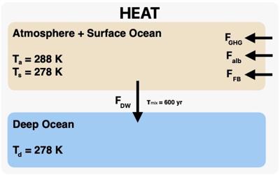
The flows of heat and preindustrial temperatures of the two ocean boxes.
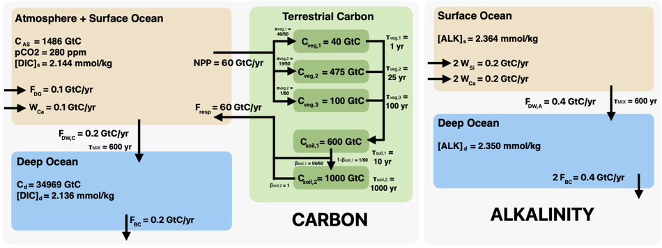
The flows of alkalinity, expressed below in terms of equivalent mass of carbon, are from weathering of terrestrial silicates and carbonates to the surface ocean, downwelling from the surface ocean to the deep ocean, and burial of carbonates on the ocean floor. The flows of carbon are the most complicated. The surface ocean and atmosphere gain carbon from degassing (e.g., volcanoes) and from the weathering of terrestrial carbonates, and they lose carbon via downwelling to the deep ocean. The surface oceana and atmosphere also lose carbon through the net primary productivity of terrestrial vegetation and gain carbon from respiration in soils. The movement of carbon between vegetation and soil pools is governed by decay timescales and preindustrial stocks that can be set by the user. Finally, the deep ocean loses carbon via burial of carbonates on the ocean floor.
The flows of heat and preindustrial temperatures of the two ocean boxes.
The physics governing the flows of heat, carbon, and alkalinity are described in the pages below.
By default, the terrestrial carbon scheme contains three pools of live vegetation and two soil pools. The number of vegetation and soil pools can be modified at runtime, but the default settings are designed to approximate the flows, stocks, and turnover times of carbon in Earth’s vegetation and soils.
Conceptually, the movement of carbon through these pools is handled by Longterm as follows. The global net primary productivity (NPP) is a function of the atmospheric CO2 concentration, and fixed fractions of that NPP flow into each of the respective pools of vegetative carbon. Each of those pools has a residence time for its carbon, with the rate of outflow (representing shedding and mortality) governed by first-order kinetics. The vegetative carbon pools operate in parallel, each receiving its designated fraction of NPP and each losing carbon at a rate proportional to its stock.
Although global NPP is specified as a function of atmospheric concentration of CO2, the fraction of NPP that goes to each vegetation carbon pool is fixed. For example, in the default preindustrial steady state, 1 PgC/yr out of 60 PgC/yr total NPP goes to the 100-year carbon pool; therefore, whatever the value of the global NPP evolves to be in the climate simulation, 1/60 of the NPP will flow to that 100-year pool. The governing equation for the mass of carbon in vegetation pool \(i\) is
The first term on the right-hand side represents the net fixing of carbon by the vegetation through photosynthesis, with \(\alpha_{\mathrm{veg},i}\) being the fraction of NPP destined for carbon pool \(i\) (e.g., 1/60 for the 100-yr pool in the default configuration). The second term on the right-hand side represents the movement of carbon from live biomass to dead biomass via plant mortality and shedding of leaves, branches, and similar material.
| Default Timescale (yr) | Default PI Carbon (GtC) | Default PI NPP (GtC/yr) | Represents |
|---|---|---|---|
| 100 | 100 | 1 | Boreal forest’s slow pool |
| 25 | 475 | 19 | Tropical and temperate forests’ slow pools |
| 1 | 40 | 40 | All forests’ fast pools |
The net primary productivity (NPP) is a function of the atmospheric CO\(_2\) concentration,
where [CO2] is the atmospheric concentration of CO2, [CO2]0 is the corresponding preindustrial value, and NPP0 is the preindustrial net primary productivity. The maximum NPP achieved when the CO2 concentration is high enough to not be a limiting factor. The preindustrial value of net primary productivity, NPP0, is determined by summing the preindustrial vegetation carbon masses divided by their decay timescales. As NPP deviates from NPP0, it is apportioned among the vegetation carbon pools in the same proportions.
Although the vegetative pools operate in parallel, the soil pools operate in serial. All vegetative pools decay to the first soil pool, which represents a combination of woody debris, litter, and near-surface soil. The loss of carbon from that soil pool is governed by first-order kinetics with a residence time that is sensitive to the global mean temperature Ts. The outflows from the soil pool are partitioned into two destinations: a constant fraction of the outflow is oxidized and sent directly to the atmosphere, with the remaining outflow sent to the next soil pool. This cascade continues to the last soil pool, which sends all of its outflow of carbon to the atmosphere.
The rate at which soil carbon decays, moving to the next soil pool and/or to the atmosphere as CO2, is set by a timescale \(\tau\)soil that depends on global-mean temperature according to a Q10 value,
with a default value of Q10 = 1.5 and with default values of \(\tau\)soil,0 for each soil pool as given in the table below.
| Default Timescale (yr) | Default PI Carbon (GtC) | Default Fraction that Decays to Atmosphere |
|---|---|---|
| 1000 | 1000 | 1 |
| 10 | 600 | 59/60 |
Terrestrial weathering of carbonate and silicate rock is represented by Fwc and Fws, which are the rates of carbon consumed from the atmosphere by the weathering of carbonate and silicate rock, respectively. These rates are dependent on temperature as
where Fwc,0 and Fws,0 are the preindustrial weathering rates, Tsurf,0 is the preindustrial surface-ocean temperature, and ac and as are the rates of relative change in the weathering rates per degree of warming (set by constants$dFwcdlogT and constants$dFwsdlogT with default values of 0.10/K and 0.02/K, respectively). Since the global mean surface-air temperature is set diagnostically as the surface-ocean temperature plus a fixed increment, these equations are identical to
The rate of carbon burial on the ocean floor in the form of calcium carbonate, \eqn{F_{bc}}{F_bc}, is linear in the concentration of deep-ocean carbonate ion,
where [CO32-] is the concentration (with dimensions of mol/kg) of carbonate ion in the deep ocean, [CO32-]0 is its preindustrial value, and a is a constant set to 2.5 x 10¹⁷ kg/yr.
The committed sea-level rise (CSL; dimensions of m) is the sea-level anomaly relative to preindustrial to which the ocean would equilibrate if the global-mean temperature anomaly were held constant. The CSL is approximated as linear in global-mean temperature with a default slope of 6 m/K. The sea level anomaly (SL; dimensions of m) is the sea-level relative to preindustrial. The evolution of SL is approximated as a relaxation towards CSL with a timescale \(\tau\)SL,
where SLmax is the maximum sea-level anomaly. The default values of \(\tau\)SL and SLmax are 2000 yr and 60 m, respectively.
The official release of Longterm will coincide with the publication of Horst, Archer, and Romps (2025), which is currently in review. The paper provides a detailed description of Longterm’s physics and the choices made for its default parameters.
Horst, I., Archer, D., & Romps, D. M. (2025). Longterm: A simple model of Earth's long-term climate. Geoscientific Model Development. (in review)@article{horst2025,
author = {Horst, Isabel and Archer, David and Romps, David M.},
title = {Longterm: A simple model of Earth's long-term climate},
journal = {Geoscientific Model Development},
year = {2025},
note = {In review}
}TY - JOUR
AU - Horst, Isabel
AU - Archer, David
AU - Romps, David M.
TI - Longterm: A simple model of Earth's long-term climate
T2 - Geoscientific Model Development
PY - 2025
N1 - In review
ER -